Trying to break a calibrated predictor
A small example of what a calibration curve can miss.
If a model says 70%, I expect the event to happen about 70% of the time among examples getting that prediction. I also want to know whether that holds for different groups within those examples.
Those two checks can disagree by quite a lot. Here’s an example where the usual calibration error is exactly zero, but the model overpredicts for one group and underpredicts for the other. Everything is small enough to calculate by hand.
One score
Take two streams of binary outcomes, A and B. An outcome is either 0 or 1. In A, the probability of a 1 is 20%. In B, it’s 80%. Draw from the streams equally often and predict 50% for everything.
The mixture has an event probability of 50%, so the prediction is calibrated. Formally, calibration means
P is the predicted probability and Y is the outcome. The only score here is p = 0.5, and the expected outcome among examples receiving it is also 0.5. But split the examples by stream:
| Stream | Event rate | Gap |
|---|---|---|
| A | 20% | −30 pp |
| B | 80% | +30 pp |
| Combined | 50% | 0 pp |
The gap is the event rate minus the prediction, in percentage points. A gets predictions 30 points too high; B gets predictions 30 points too low. Averaging the two gaps gives zero.
For the rest of this example, assume we know the stream before making a prediction. We could then predict 20% for A and 80% for B. That predictor is calibrated too. The difference is that it uses information the constant predictor throws away. Without the stream identifier, we’d need another feature that lets us tell the cases apart.
Three scores
The constant prediction makes this particularly easy to arrange. The construction also works with several scores.
Use three scores: 20%, 50%, and 80%. At each score, include equal numbers of A and B examples. Set A’s event probability 15 percentage points below the score and B’s 15 points above it. A then has probabilities 5%, 35%, and 65%; B has 35%, 65%, and 95%.
Among examples assigned 20%, the average event probability is (5% + 35%) / 2 = 20%. The arithmetic works the same way at 50% and 80%. Each combined point lands on the diagonal.
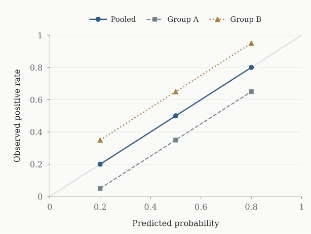
Narrower calibration bins won’t help here. An A example and a B example can have exactly the same score, so they’ll stay in the same bin however fine we make it. We have to split by group to see the two errors.
It’s also worth keeping the scores separate within each group. In a different construction, A could be overpredicted at one score and underpredicted at another. Checking just A’s average would let those errors cancel again.
Checking the arithmetic
The Python script builds 1,000 examples for each group–score pair: 2,000 rows for the constant predictor and 6,000 for the three-score version. The number of positive outcomes is fixed. A cell with an event rate of 5%, for instance, gets 50 ones and 950 zeros.
Given a score p and a gap, the two groups are constructed like this:
for group, rate in (
    ("A", p - gap),
    ("B", p + gap),
):
    positives = 1000 * rate
    rows.extend(
        (group, p, rate,
         int(i < positives))
        for i in range(1000)
    )
Each row contains the group, prediction, generating probability, and outcome. The script uses Python’s Fraction type so the checks are exact. Row order doesn’t matter.
To get a calibration error, bucket the rows by prediction and average the signed errors in each bucket. Then take the absolute values and weight them by each bucket’s share of the rows. Run the calculation again, this time bucketing by both group and prediction:
          pooled  grouped
constant  0.0000   0.3000
3 scores  0.0000   0.1500
Nothing about the predictions changed between the two columns. The first calculation lets A’s errors cancel B’s; the second takes their absolute values separately.
These exact zeros come from fixing the counts. If we sampled the outcomes instead, the observed rates would fluctuate around the probabilities above. Fixed counts make the cancellation easier to inspect, but they don’t tell us how well a fitted model would do on new data.
Brier score
The Brier score averages the squared error of the predictions. For binary outcomes:
Lower is better. The constant 50% predictor scores 0.25 because it’s half a unit away from every outcome. Predicting 20% for A and 80% for B gives 0.16. For A, that’s 0.2 × 0.8² + 0.8 × 0.2²; B gives the same answer.
In the three-score example, with equal counts in all six cells, the original predictor scores 0.19. Using the true probabilities in each cell brings it down to 0.1675. The improvement is 0.0225, or 0.15².
There’s a reason the square appears. If the event probability is q, the expected squared error at prediction p is q(1 − q) + (p − q)². Predicting q removes the second term. Here, p and q are 0.15 apart in every cell.
So Brier score can distinguish these predictors even though both pass the pooled calibration check. The improved predictor has an unfair advantage: we gave it the true probabilities. On real data, we’d have to estimate them from training data and see whether the improvement held up on a separate test set.
I wouldn’t use a lower Brier score as proof of better calibration, though. It also rewards a predictor for separating high-probability cases from low-probability ones. The scikit-learn calibration guide goes through this distinction.
Why recalibrating the score doesn’t help
Suppose we pass the constant predictor’s output through a function that adjusts its probabilities. Every input is 0.5, so a deterministic function must return the same number, q, for everyone. A needs q = 0.2. B needs q = 0.8. There’s no choice of q that works for both.
The same problem occurs at each score in the second example. A more flexible recalibration curve still sees identical inputs for A and B. It has no way to tell them apart.
If we let the function use the group, the fix is simple: subtract 0.15 for A and add 0.15 for B. We know those offsets because we constructed the data. Learning a correction from finite samples, especially across many overlapping groups, is a harder problem.
Multicalibration, introduced by Hebert-Johnson, Kim, Reingold, and Rothblum, asks for approximate calibration across a specified collection of identifiable subpopulations. Our two streams are a small example of why that extra requirement matters. The collection has to be specified: passing checks for A and B doesn’t give a guarantee for every subgroup someone might ask about later.
Changing the mixture
Go back to the constant predictor. Keep A’s event rate at 20% and B’s at 80%, but let B supply 80% of the examples instead of half.
The combined event rate becomes 0.2 × 0.2 + 0.8 × 0.8 = 0.68. Our prediction of 50% is now off by 18 percentage points. The only thing that changed was how often each stream showed up.
The Brier score stays at 0.25. Predicting 0.5 gives the same squared error for a 0 as for a 1, so changing their proportions can’t move it. That’s another reason to look at the calibration curve separately.
The predictor that uses 20% for A and 80% for B still works under this shift. It doesn’t rely on the two groups arriving equally often. It does rely on their internal event rates staying fixed; if those change too, we’d need to check again.
Checking this on real data
This example gives us the groups and their event rates in advance. On real data, I’d start by choosing which groups to check and recording how many examples fall into each group at each score. The population and time period matter too, as the mixture change above shows.
I’d keep the data used to fit a recalibration function separate from the data used to evaluate it. There’s a similar issue with searching for groups: if we keep splitting a test set until we find a large error, we may just have found an unusual sample. That group needs to be checked on fresh data before treating the gap as a repeatable failure.
Even without a search, small groups give noisy curves. For independent binary observations with probability 0.5, the standard deviation of the sample mean is 0.5 / √n. With 100 observations, that’s 5 percentage points. With 10,000, it’s 0.5 points. A five-point gap means something quite different in those two cases, and checking many groups makes uncertainty harder to handle.
Continuous predictions add a choice we avoided here: how to group nearby scores. Very narrow bins give more detail but fewer observations per bin. Arrieta-Ibarra and coauthors’ paper on calibration metrics discusses that tradeoff. In this construction, the scores are identical within each bucket, so the group errors remain even when there’s no binning approximation.
The pooled calculation checks E[Y ∣ P = p] = p. Splitting by group checks E[Y ∣ P = p, G = g] = p. In this example, averaging over G is exactly where the errors disappear.